Probability Free Response Review

We went over two AP problems in class today from the old AP exams, and I have to say, I'm very impressed at how well you guys did with them! Great job! Take those with you and be sure to study.

Of course, the best way to study stat (or any math class, for that matter) is to PRACTICE lots and lots of questions. I've found that some of the best resources are in the AP practice books that you can buy on Amazon.com. Now, if you haven't gotten around to doing that yet, a great alternative is to go to:

http://apcentral.collegeboard.com/apc/members/exam/exam_information/8357.html

The questions we did today were from the 2011 exam and the 2010 exam. When you get to this page, scroll down and you'll see the questions, full-scale answer keys, and samples of student responses. AWESOME.

There are also solutions keys to the extra examples that I gave out in class, as well as sample student responses. 5 extra points on your next test if you can guess how old I'm going to be for my upcoming birthday correctly.

Venn Diagrams and Probability Distributions

Venn Diagrams are used when an event can take on two probabilities. For example: "There are two students in statistics, 4 in english, and 5 in both." The key word "both" tells us to use the Venn Diagram. Create the Venn Diagram first, then use it to determine whatever probability the question is asking you for. Remember that anything that is "neither" goes on the outside.

A probability distribution is a chart of probabilities when the random variable, x, can take on many different values. It looks like this:

x           0     1     2     3     4
P(x)     .1    .2   .15   .1   .45

x is the random variable. The numbers next to it are the values that the random variable can be. For example, I could get into zero, 1, 2, 3, 4 car crashes per year. The bottom row P(x) tells us the probability associated with that value. For example, the probability of me getting into 2 car crashes is .15. The bottom row of probabilities must always sum to 1.

Independent Events

Independent Events are two events whose outcomes are not influenced by one another. By definition, we know that two events are independent if the probability of one event happening is the same as the probability of it happening given a second event. Your AP formula sheet writes it like this:

P(A) = P(A | B)

In plain english, this means that we have two events, A and B. On one side of the equation, we calculate the probability of event A happening. On the other side of the equation, we calculate the conditional probability of event A, given that event B has already happened. If they are the same on both sides of the equation, then we have independent events. If not, then the events are dependent on one another.

In context, "independent events" means that whatever event B is does not influence or change the probability of event A when it happens. For example, if a student of mine skips class to go watch a fight, that's not going to change the probability that I'm still going to be teaching class that period. So the student going to the fight and me teaching class would be independent events.

"Dependent events" means that event B somehow influences the outcomes of event A. Therefore, the probability of them happening together is different than if event A happened by itself. For example, the probability of me showing up to teach on a given day is probability about 98%. However, the probability of me showing up to teach given that I know I have a cold is significantly lower, probability around 30%. So since p(teaching) does not equal P(teaching given cold), those two events would be dependent on one another.

Hints for Problem Set 4 (Probability)

Problem 1:
The key to this question is effectively defining your sample space by making a correct tree diagram. Think CAREFULLY about what your random variables are in this case, and remember that you need a new level of your diagram for each random variable.

For parts B and C, find your key words in the question. Recall that some key words tell you to multiply while others tell you to add.

Problem 2:
As in the last one, make a good tree diagram. NOTE that we are selecting two books and that our events are 1) selecting the first book and 2) selecting the second book. Overnight/renewing are not events in this case because, according to the question, we need to be picking two books, one right after the other.

Problem 3:
Remember that I forgot the "A" in part iii - whoops!

For this one (part iii), you can show your work either by explaining the tree diagram or by showing how you used the intersection rule effectively. Either one will receive full credit, just be sure to write out your probability statements.

Problem 4:
Think about the properties of decks of cards. There are 52 cards, 13 cards per suit, and 4 suits. ALL of the suits are equivalent to one another other than the fact that they are hearts, spades, clubs, and diamonds. If you write a knock knock joke on the last page of your problem set then I will give you five bonus points. So then, numerically, should anything about them be different? Hmmm.....

Problem 5:
Part a: the probability is not 1/6 per each face because the dice is loaded. You're going to have to change the denominator for this one. This question is probably the hardest one on the problem set...

Part B and C: once you have part A figured out, these two should be no problem at all

Part D: Don't let the notation throw you off on this. Just think carefully about what the question is asking you. Just like number one, you're going to need a new denominator for this question, too. Once you find it the rest of the problem should be pretty straightforward.

Good luck!

Conditional Probability

Conditional Probability means that we must have two events - call them event A and event B (or whatever two random variables exist in your problem). Given that one event has already happened, or given that one random variable is present, what is the probability that the other will also happen? Or what is the probability that the other random variable will also exist?

Your AP exam formula sheet gives you the conditional probability theorem like this:

This is read as, "The probability of A, given that B has already happened." This is equal to the probability of A and B (numerator) over the probability of B (denominator), where B is the event that already happened.

We usually use a 2-way contingency table when finding conditional probabilities. Find the marginal totals (row and column totals) first. Then, you will use these totals along with the information within the table to find your conditional probabilities.

Probability Rules

We have five basic probability rules that we must follow when determining the probability of an event or events. Say we have a random event x or two random events x and y. The five basic probability rules are:

1. All probabilities must be between 0 and 1. We can't have anything greater or less, because that doesn't make sense.
0 < P(x) < 1

2. Probabilities that don't have any outcomes in common are said to be DISJOINT or MUTUALLY EXCLUSIVE.

3. Complement probability is the opposite - the probability if it doesn't happen.
P(not x) = 1 - P(x)

4. Multiplication Rule (union): Probability of x AND y happening at the same time.
P(x and y) = P(x) times P(y)

5. Addition Rule (intersection): Probability of x OR y happening, but not both of them at the same time.
P(x or y) = P(x) times P(y) - P(x and y)

Stat Test and Hints for Problem Set #3

We took our stat test today. The highest grade was an 84% and it was actually achieved by multiple students - nice job! The lowest grade was a 23%. If you want to ZAP a test that's completely fine, but remember, you have to STUDY first. Good grades in classes (ESPECIALLY college level classes) don't happen by pure luck. Actual effort is involved.

Below are some hints that you might find helpful for the problem set that's due tomorrow:

Problem1:
Part A: Only one answer is correct. The other three are false. Full credit will be provided to those who give an explanation WHY.
Part B: This is a GREAT question - really shows if you understand std. dev. or not. You must pick 4 numbers between 0 and 10. They can be the same, or different. Basically, I want to know that, in order to minimize std. dev (so sx is as small as possible), what should all your numbers be that you're picking? What must be true about these four numbers to make the std. dev. small? Remember, std. dev. is the distance from the mean - the more different your numbers are, the bigger your std. dev. becomes....
The reverse is true for making the std. dev. as large as possible.
Part C: A "resistant measure of spread" means that, if we stuck an outlier into the data set, the spread wouldn't really change much/at all. Recall that the IQR is the middle 50% of the data....
Part D: Remember that means are calculated by adding up all the numbers and dividing by how many there are. That doesn't necessarily mean that there must be equal amounts of men and women in this company.

Problem 2:
Another GREAT question. Think of a graph that you can make with the given information (for both male and female doctors) that would help you to determine the shape of the data. Hint: it's NOT a Normal Curve. Why? Well, just because we have a mean and a std. dev, that doesn't imply normality. EVERY quantitative data set in the world has a mean and a std. dev, but that doesn't imply that EVERY data set is also symmetrical (which the Normal Curve is). So, given all that information, what other graphs can be created?

Problem 3:
Part a: Find the standard deviation using the formula we used in class. There should be an example of this in your notes.
Part b: Remember how to interpret: also in your notes. IN THE CONTEXT OF THE PROBLEM! INCLUDE UNITS FOR FULL CREDIT.
Part c: This one you should be able to figure out on your own, but my advice is to BE SPECIFIC. A one-sentence answer isn't going to cut it here.

If you write I love Math at the top of your problem set tomorrow I will give you 5 bonus points.

Problem 4:
Part a: TITLE, LABELS, AND SCALE
Part b: CUSS
Part c: Think about the shape of your boxplot in regards to what we talked about in class
Part d: Again, be specific. More would change than just the spread of the data, although that's certainly part of it. Remember to tell me WHY along with the WHAT.

Problem 5:
Graphically means make some type of graph that makes sense given the type of data. Numerically means 5-number summary. Summarize your findings means write a paragraph, using SPECIFIC language, units, and such to talk about what you SEE.

Good luck!

For those who were on the Constitution Field Trip today....

Q: "Do I have to take my test tomorrow?"
A: Yes. You've known about it for roughly a week. Be on time tomorrow. The test is in the lecture hall.

Q: "How can I study for the test?"
A: 1) Review your notes and examples. Going online might also help you fill in the gaps where you don't understand.

2) Review the notes posted in this blog.

3) Do your review sheet that's due on Wednesday. The problems on it will help further your understanding of the statistical concepts. And if not, then make sure you ask me questions.

4) Come by my room and get some practice questions. I have both practice multiple choice and open response. Also, feel free to come by room 120 after school for some tutoring.

Review for the Chapter 2 Test (Numerical Measures of Data)

Here are 10 important things that you should know how to do in order to be successful on the test tomorrow:

1.How to find a mean/median on a graph (and WHICH graphs contain mean/med)
2.How to determine a median from a frequency table
3.How to locate quartiles on a graph
4.How to calculate outliers using the 1.5 outlier test
5.How the mean/median/IQR/standard deviations CHANGE when taking outliers out of a data set
6.The difference between IQR and range
7.How to determine shape of a distribution from a graph, particularly boxplots
8.Standard deviation: what it is and what properties it holds
9.How to calculate a z-score
10.How to use z-score to estimate a percentage on a Normal curve

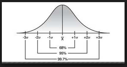
One thing that we talked about today that was not mentioned previously is called the Empirical Rule, or the 68-95-99.7 rule. It states that 68% of the data on a Normal curve should fall within the first standard deviation, 95% of the data should fall within the 2nd std. dev, and 99.7% should fall within the 3rd std. dev. Anything outside is considered an outlier (beyond 3 std. dev, so in other words, we would expect the z-score for an outlier to be above 3.0 or below -3.0)

See the picture below for more detail:

Normal Quantile Plots

Previously, we talked about z-scores and how they tell position on the Normal Curve - but how do we know if the data fits a Normal Distribution in the first place? A Normal Quantile Plot (also sometimes called a Normal Probability Plot) can give us an idea of Normality of the data. Put your data into L1, then go to Stat Plot and choose the very last graph. Don't forget to go to zoom - 9(stat) to get a good view of your graph!

We look for three characteristics of the data to assess Normality. 1) Does the data roughly form a straight line? Or do we see curvature at the ends? 2) Is the data centered about the x-axis - do we see roughly equal observations above and below? And finally, 3) Does a majority of the data appear to be in the middle of the graph rather than in the tails? If the answer to these 3 questions is "yes" then we can assume that our data appears roughly Normal.

Note that this is our ASSUMPTION based on our OBSERVATIONS. We didn't actually PROVE anything with our Normal Quantile Plot. Choose your language carefully when you interpret this.

Normal Curve and Z-Scores

The Normal Curve is otherwise known as the bell curve. It is a symmetric distribution centered about the mean and spread out by standard deviations. 68% of the data lies within the first standard deviation. 95% lies between the first two standard deviations. And 99.7% of the data falls within the first 3 standard deviations.  Anything outside of the first three standard deviations is considered an outlier of the data (which means that 0.3% of the observations will be outliers).

To calculate position on the Normal curve, we can use the z-score formula, which is the sample mean minus the population mean, all over the standard deviation. Our answer (the z-score) can be interpreted as the number of standard deviations (positive or negative) above or below the mean.

Standard Deviation

The standard deviation is how far away each observation is, on average, from the mean of the data. We use standard deviation as a measure of spread about the mean, just as we use the interquartile range as a measure of spread about the median. Standard deviation, as paired with the mean, is typically used in symmetric or roughly symmetric data sets.

We can calculate the standard deviation using a long formula, or we can simply find it in the calculator when we do a 5-number summary (1-var statistics). Don't forget to always interpret it in the context of the problem!

Guest Speaker from Fayetteville

Dr. Watson, a petrochemical engineer from the University of Arkansas, stopped by the library today to talk about a two-day trip opportunity. He also discussed ACT score and how important it is to the college application process. You need a 19 to get into the University of Arkansas unconditionally, and 18 to get in with remediation classes.

Remember, I do after school ACT prep from 3:40pm - 5:40pm in Mrs. Cain's room - 120. We cover all the subjects: Mrs. Cain does English and reading, I do math and science (aka how to read graphs properly). Come and join us - practice makes perfect!

Shout out to Nakeya and Antonia for coming after school today, and shout out to Trey and Megan for ZAP-ing their tests for a better grade.

Hints for Problem Set #2

Problem 1A: Think about what type of data is displayed in a histogram, and think about how many random variables that Mrs. Timmons is trying to work with. For part three, I'm asking what features she might see in the histogram IN GENERAL. I didn't provide you with one. But if she was looking at a histogram, what would she see? Think: CUSS....and go from there.

Problem 1C: Think about the shape of the histogram: given this specific shape, which estimate should be higher, the mean or the median? Check your notes from Friday, August 30th if you're stuck. I'm looking for an approximation here, there's no "right" answer as long as you justify it properly in part B.

Problem 1D: How can we measure center? There is, as we know from our notes from August 30th, more than one way....

Problem #5: Assume that you're taking the median of the 6 existing weights of luggage - that is, don't count x7 just yet. Otherwise, you're not going to be able to start the question.

Thursday and Friday: Cities Survey/Experiment

Does giving a point of reference increase accuracy in estimation? Students worked in partners to explore this effect. Each group chose a city, then asked 15 different people (each): how many people do you think live in this city? OR, How many people do you think live in this city, given the 2010 population?

Most groups should have found that their data is more spread out without giving a reference point. When we throw in a reference point (otherwise known as an "anchor"), people then have grounds in which to base their estimation. Otherwise, they are relying solely on their prior knowledge of the city when making an estimation.

Students then turned in 7 questions about their findings. One key point to reinforce is that, when given symmetric data, use the mean as a measure of spread. When given skewed data, use the median as a measure of spread.

Shout out to Issac Wilburn and Josh Reynolds for working with remarkable intensity during the entire class period on Friday!

Boxplots and the 1.5 Outlier Test

Boxplots display univariate, quantitative data. The data is ordered and placed into quartiles. Quartiles 1 and 4 are represented by the whiskers, and quartiles 2 and 3 (called the Interquartiles, since they represent the middle 50% of the data) are represented by the boxes.

We can CUSS about the boxplot because they show center (the median), outliers (via the 1.5 outlier test), shape (look for symmetric versus skewed), and spread (look at the range or the interquartile range).

Problem Set 2 was given out in class today. Check tomorrow's blog post for hints for question 1.